April 2026
Efficient division-free randomness extraction
1. Introduction
This post introduces an approach for randomness extraction from sequences of independent observations from an unknown but unchanging probability distribution (including coin tosses, dice rolls, thermal noise observations, ...). It only requires basic arithmetic ($+$, $-$, $\times$) and a count trailing zeroes (ctz) operation on fixed-width integers, and can be implemented without table lookups or other timing side-channels. Variants are provided for binary and multi-valued input symbols. We analyze how much entropy it can extract, and its performance.
The techniques here may be useful to cheaply reduce the amount of data that needs to be fed as seed input to a CSPRNG. Variants of it can also be used as the basis for human entropy generation approaches.
1.1. Von Neumann extractors
Randomness extraction is the problem of turning a stream of symbols sampled i.i.d. from an unknown probability distribution (such as many throws of the same, potentially unfair, coin or die), into a stream of perfectly uniform bits. Consider the following algorithm:
- Loop:
- Toss the same coin twice, and if:
- heads+heads (HH): output nothing
- heads+tails (HT): output 0
- tails+heads (TH): output 1
- tails+tails (TT): output nothing
- Toss the same coin twice, and if:
This is the Von Neumann extractor[1]. Let $p$ be the (unknown) probability of tossing heads. The probabilities of HH and TT are $p^2$ and $(1-p)^2$ respectively, which we cannot reason about without knowing $p$. But HT and TH both have probability $p \cdot (1-p)$. Thus, we can just use these two cases, and produce one bit of output for them, which will have exactly equal probability of being 0 or 1. The other cases are discarded.
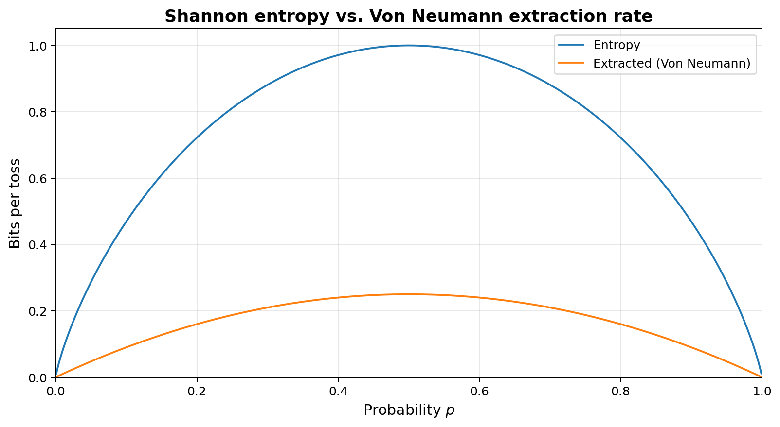
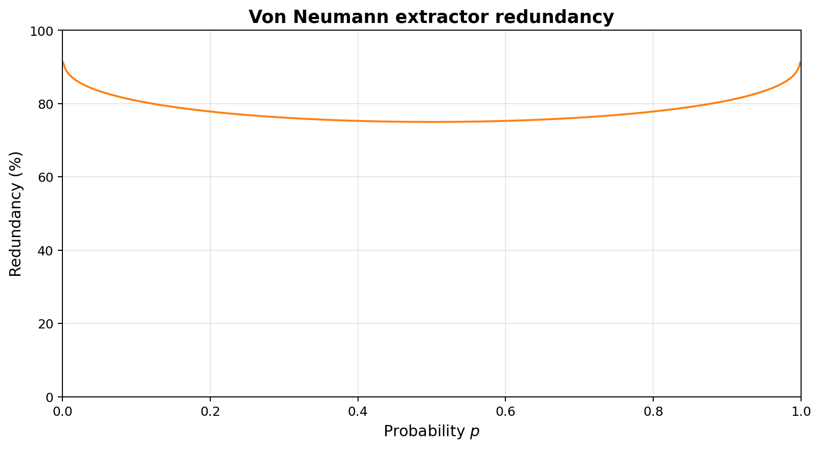
In the best case, when the coin is actually fair ($p=1/2$), this extractor outputs 0.25 bits per toss, while the input tosses have a Shannon entropy of 1.0 bits per toss (the upper bound on the amount of entropy that can be extracted), so we have a redundancy of 75%. When the coin is biased, say $p=1/4$, the entropy drops to 0.811 bits per toss, but the extracted amount drops further to 0.1875, or a redundancy of 76.9%. As the coin grows more biased, the redundancy increases further, approaching 100% at the edges ($p=0$ or $p=1$).
1.2. Peres extractors
One can reduce the redundancy by extending the extractor with two extra output streams, $U$ and $V$, which are not uniform (unlike the normal output), and feeding those as input into new extractors. This is the Peres extractor[2]:
| Tosses | Output | U | V |
|---|---|---|---|
| HH | - | E | H |
| HT | 0 | D | - |
| TH | 1 | D | - |
| TT | - | E | T |
$U$ reports E or D, depending on whether the two tosses were (E)qual or (D)ifferent. $V$ reports what the input tosses were if they were equal. The normal output is the only guaranteed-uniform one, but the combination of Output, U, and V, fully determines the input, so no entropy was lost. In the fair case, the output will have 25% of the entropy, and $U$ and $V$ will have 50% and 25% of the entropy.
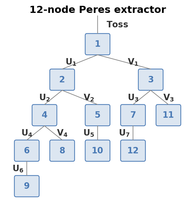
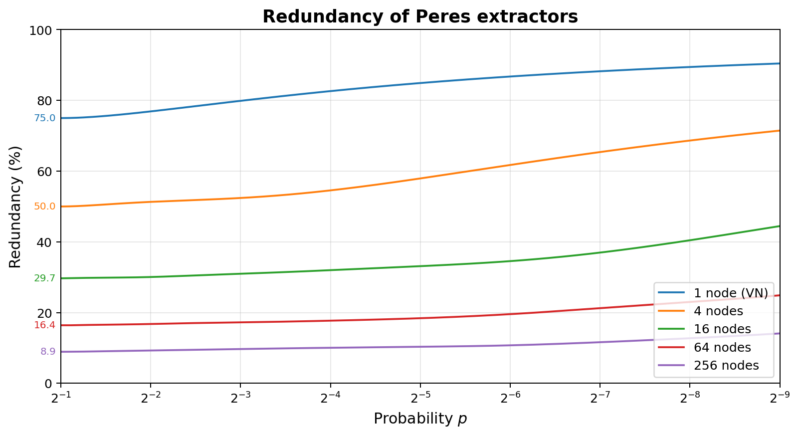
When building a tree with a given number of nodes, one should generally place nodes where the most expected entropy is, and break ties by minimizing the number of $V$ edges above, as their relative entropy decreases compared to $U$ edges as bias increases. This explains the skewed tree in the diagram above, which also labels each node by decreasing quality. The plot on the right shows the redundancy of this approach with 1, 4, 16, 64, and 256 nodes.
These extractors are extremely simple to build in hardware, as they only need 2 bits of state per node: whether the node has seen an odd or even number of inputs, and in case of an odd number, what the last input was. They are also relatively robust against biased input. A downside is that they are inefficient in software, very hard to implement in a way that does not leak secret information through runtime, and the amount of state needed to approach perfect extraction grows quickly. Asymptotically, one needs $\approx 1.035 \times r^{-2.27}$ nodes as the redundancy $r \rightarrow 0$, or halving the redundancy means approximately $4.83$ times more nodes.
1.3. Elias extractors
It is possible to improve upon the Von Neumann extractor in a different way[3]. Imagine we do not look at groups of just two tosses, but larger numbers, for example 5. We can then group them by counts of heads/tails, because different outcomes with the same numbers of heads and tails have identical probability. For example, all 10 cases with two heads and three tails have probability $p^2 \cdot (1-p)^3$.
| heads/tails | tosses |
|---|---|
| 5/0 | HHHHH |
| 4/1 | HHHHT, HHHTH, HHTHH, HTHHH, THHHH |
| 3/2 | HHHTT, HHTHT, HHTTH, HTHHT, HTHTH, HTTHH, THHHT, THHTH, THTHH, TTHHH |
| 2/3 | HHTTT, HTHTT, HTTHT, HTTTH, THHTT, THTHT, THTTH, TTHHT, TTHTH, TTTHH |
| 1/4 | HTTTT, THTTT, TTHTT, TTTHT, TTTTH |
| 0/5 | TTTTT |
In case of 5 heads or 5 tails, no information is gained, because there is only one combination in that class. But in the other classes, there are many combinations, and they can be mapped to bit sequences. For example, of the 5 combinations for 4/1 and 1/4, one can assign uniform 2-bit outputs to 4 of them, and discard the 5th combination. One can also assign 3-bit outputs to 8 out of the 10 combinations for 3/2 or 2/3, and separately assign 1-bit outputs to the 2 remaining combinations. In general, the number of elements in each class is a binomial coefficient $\binom{n}{k}$, and it gets split up into a sum of powers of two, each of which is turned into the corresponding number of bits.
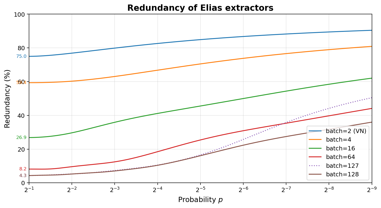
Like with Peres extractors, as the number of observations per batch goes up, the redundancy approaches 0%, and does so faster than Peres with increasing nodes, needing batches of size $\approx \log_4(1/r) / r$ as the redundancy $r \rightarrow 0$. Due to the behavior of splitting up classes of outcomes into groups with a power-of-2 size, larger batches are not necessarily better than smaller batches. This is demonstrated here for 127 and 64, where the difference is very pronounced for biased input.
Elias' approach can be straightforwardly generalized to multi-valued inputs (e.g. dice, or multiple measurement levels for thermal noise). One considers the number of distinct permutations of the seen observations, whose class sizes become multinomial coefficients rather than binomial coefficients, but the rest of the approach remains unchanged: assign uniform bit outputs to each permutation within a class of equal-count observations.
A downside that Elias extractors have is that implemented naively, one needs tables to convert the different toss observations to bits, and the size of those tables grows exponentially with the batch size. Ryabko and Matchikina[4] (RM) introduced an algorithm for computing these bit patterns without tables. Formulas exist for computing the position of a sequence of heads/tails observations in the lexicographically-ordered list of observations with the same counts. These can be evaluated relatively efficiently, though this involves multiplications and divisions with possibly large integers. That position can then be converted to a uniform bit pattern.
2. Improvements
In this section, we will improve upon the RM approach in a number of ways:
- Improve efficiency by carrying state from one batch to the next, avoiding the need to produce a fixed number of bits per batch.
- Extend support to multi-valued inputs without precomputed tables.
- Improve efficiency, using fixed-size integer arithmetic without division operations.
- Make the algorithm deal with integer overflow, hurting redundancy but not correctness.
- Make runtime optionally independent of the entropy produced, making it usable in security-critical settings.
The following subsections introduce the algorithm step by step.
2.1. Restating the RM approach
To have a baseline to start building upon, let us first present the RM approach in an algorithmic fashion.
It consists of two steps:
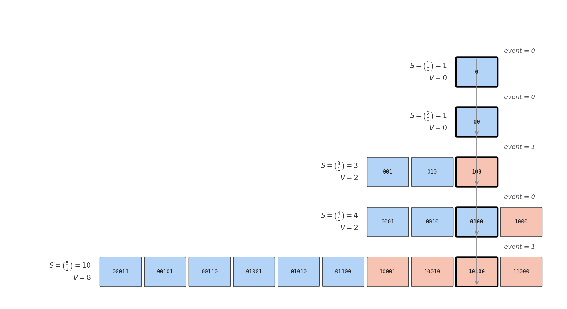
- Given a batch of $n$ boolean events of which $k$ are $1$ and $n-k$ are $0$, compute span $S = \binom{n}{k}$, the number of ways these could have been ordered. Further compute value $V \in [0, S)$, the position the actually observed order has within a lexicographically sorted list of all these orderings.
- Convert this $(S, V)$ pair to a sequence of uniform bits.
2.1.1. Mapping batches to uniform spans
The position in the lexicographic ordering can be computed recursively. Among the $\binom{n}{k}$ possible values, we must place the $\binom{n-1}{k}$ which start with a $0$ first, followed by the $\binom{n-1}{k-1}$ which start with a $1$. Unsurprisingly, these two classes form exactly a proportion $\frac{n-k}{n}$ resp. $\frac{k}{n}$ of the entire span: when one has $n-k$ zeroes and $k$ ones, the number of combinations that start with a zero resp. one will be proportional to $n-k$ and $k$.
Thus, if one has already computed the $(S, V)$ for the later $n-1$ events, those for all $n$ events can be calculated by:
- Scaling the span $S$ by $\frac{n}{n-k}$ (if event is 0) or by $\frac{n}{k}$ (if event is 1).
- If the event is 1, adding $\binom{n-1}{k}$ (the number of combinations with the same $k$ starting with 0) to the value $V$. This is exactly the difference between the old and the new span.
By unrolling the recursion, and reversing the order of events (meaning we find the position in the reverse-lexicographic ordering instead), we get:
def process_batch(events: List[bool]):
    """Compute (span, value) for a batch of binary events."""
    # Number of True events so far.
    k = 0
    # Base case for empty list.
    span, value = 1, 0
    # Process events one by one:
    for n, event in enumerate(events, start=1):
        k += event
        num_equal = k if event else (n - k)
        new_span = (n * span) // num_equal
        value += event * (new_span - span)
        span = new_span
    return [span, value]
2.1.2. Mapping uniform spans to bits
For reasons that will become clear later, it is desirable to restate the conversion to bits as an operation that potentially extracts a single bit from a $(S, V)$ pair, which can then be applied repeatedly.
Whenever $S$ is even, there are exactly as many even values as odd values. Thus, in this case we can shift down both $S$ and $V$, and return the original bottom bit of $V$ as uniform output bit. Whenever $S$ is odd however, there is one value which cannot be paired with another. For this one value we must reset the state and return nothing to remain uniform.
def extract_bit(uniform) -> bool | None:
    span, value = uniform
    # Deal with odd spans.
    if span & 1:
        # Map last value in span to nothing.
        if value == span - 1:
            uniform[0], uniform[1] = 1, 0
            return None
        # The last value in the span was removed.
        span -= 1
    # Extract bottom bit
    ret = bool(value & 1)
    uniform[0], uniform[1] = span >> 1, value >> 1
    return ret
The combination of using process_batch on a batch, followed by repeatedly invoking extract_bit until it returns nothing anymore, is exactly
equivalent to the Elias extractor, in terms of the probability distribution of produced outputs.
2.2. Multi-valued inputs
The algorithm can be extended in a relatively straightforward manner to deal with multi-valued inputs, at the cost of additional computation cost. Instead of binomial coefficients, one needs multinomial coefficients. Let $m$ be the number of possible events, and let $f_i$ be the number of occurrences of event $i$. This means $n = \sum_{i=0}^{m-1} f_i$, as every event is one of the possible values. The total span $S$ is now $\binom{n}{f_0, f_1, \ldots, f_{m-1}}$.
Like before, this can be computed recursively. If one has computed the span $S$ for the later $n-1$ events, the one for all $n$ events is a factor $\frac{n}{f_s}$ larger, where $f_s$ is the frequency of the current symbol. We can no longer use the trick of adding the difference between new and old $S$ for offsetting the value $V$, but must instead compute how many combinations that lead to the same frequencies exist which start with an event lower than the current one. This too is a rescaled version of the old span $S$, with a factor $\frac{\sum_{i=0}^{s-1} f_i}{f_s}$.
Applying the same unrolling and reversal as before:
def process_batch_multi(events: List[int]):
    """Compute (span, value) for a batch of multi-valued events."""
    # Number of events per value so far.
    freq = [0 for _ in range(m)]
    # Base case for empty list.
    span, value = 1, 0
    # Process events one by one:
    for n, event in enumerate(events, start=1):
        freq[event] += 1
        num_equal = freq[event]
        num_below = sum(freq[:event])
        new_span = (n * span) // num_equal
        value += (num_below * span) // num_equal
        span = new_span
    return [span, value]
This process_batch_multi acts as a drop-in replacement for process_batch, usable when the input data is not binary, for example
when rolling a die, or when measuring multiple levels in thermal noise (though only when one can guarantee the samples are
independent).
The downside is that it requires two division operations (which we will get rid of later, but some extra cost remains) per event, and $\mathcal{O}(nm)$ additions.
2.3. Carrying state across batches
One non-trivial source of redundancy in all these approaches is the fact that the resulting $(S, V)$ needs to be fully converted to bits for every batch. This is a waste of entropy, because the smaller the span $S$ gets, the higher the fraction of states for which the odd-last-value case triggers. However, the $(S, V)$ representation can support aggregation of multiple such uniform spans:
def merge(uniform1, uniform2):
    """Combine the entropy from two sources."""
    span1, value1 = uniform1
    span2, value2 = uniform2
    return [span1 * span2, value1 * span2 + value2]
With this, it becomes possible to continuously update a single global state, merging data from new batches coming in, and extracting bits whenever the state grows too large. For example, one can carry $c$ bits of state across batches, reducing the probability of hitting the odd-last-value case to at most $2^{-c}$ per batch.
state = [1, 0]
while True:
    batch = receive_events()
    new_data = process_batch(batch)
    state = merge(state, new_data)
    while state[0].bit_length() > c:
        bit = extract_bit(state)
        if bit is None: break
        output(bit)
This approach has some similarity to entropy coders like range coding and asymmetric numeral systems (ANS)[5]. Like ANS, it works with growing integers rather than shrinking ranges. Like range coding, it tracks both a value and a span, which are needed to guarantee absolute uniformity. Unlike both, certain states can be reached in which all information is thrown away when extracting bits, if doing so cannot be done perfectly. This is of course unacceptable when trying to reversibly compress data, but the only option in our setting.
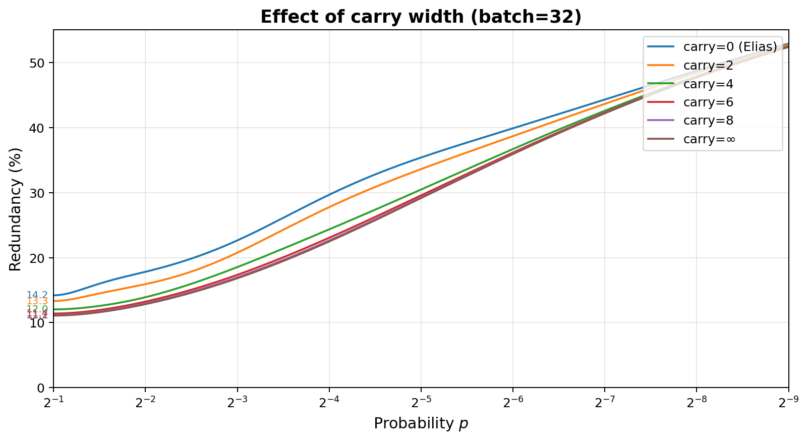
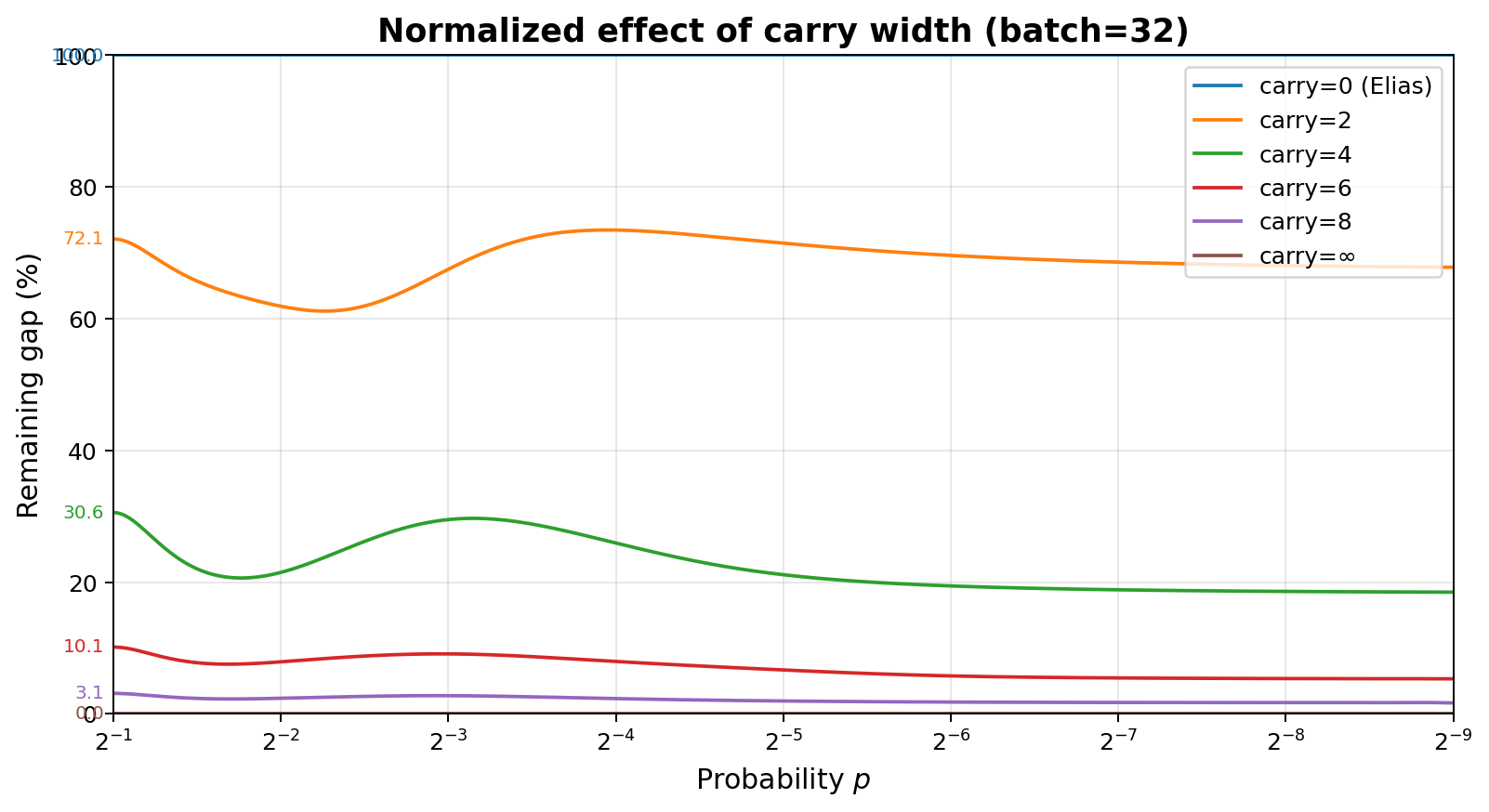
This graph shows the benefit of carrying 0, 2, 4, 6, 8 bits, and the limit as the number of carry bits goes to infinity. The right graph shows the same data, but normalized so that 100% corresponds to 0 bits of carry, and 0% corresponds to $\infty$ bits of carry. No carry is equivalent to Elias. It shows how even just 8 bits of carry reduces the redundancy gap to approximately $1/32$ of the no-carry case in this example.
2.4. Fixed-width arithmetic
On real hardware, operands of arithmetic operations are limited in width. Arithmetic operation results are generally truncated to $B$ bits, effectively computing values modulo $2^B$. When overflow occurs, this means results will be incorrect. Thus, one must limit batch sizes to $n$ such that $n\cdot\binom{n-1}{k} < 2^B$ for any $k$. This means the following limitations:
| Bit width | Max batch size |
|---|---|
| 8 | 7 |
| 16 | 15 |
| 32 | 30 |
| 64 | 62 |
| 128 | 125 |
We use two approaches to weaken this restriction.
2.4.1. Avoiding divisions
Division instructions are undesirable for multiple reasons:
- They are relatively slow compared to multiplications, thus avoiding them is generally a good idea for efficiency reasons.
- They are often variable-time in hardware, making them inappropriate when timing attacks are relevant.
- They are not compatible with the overflow-resistance technique described in the next section.
To avoid divisions in the process_batch and process_batch_multi,
we can rely on the fact that all divisions are whole: the result is always an integer again. This means divisions
by odd numbers can be written as multiplications with their modular inverse (modulo the range of the word type,
for example $2^{64}$ for $B=64$), which is not hard to compute using Newton's method[6]:
uint64_t mod_inverse(uint64_t x) noexcept
{
    // 4-bit-correct seed via a branch-free table trick.
    uint64_t inv = x ^ (((x + 1) & 4) << 1);
    // Newton's method: each iteration doubles the number of correct bits.
    for (int i = 0; i < 4; ++i) {
        inv *= 2 - inv * x;
    }
    return inv;
}
In addition, divisions by powers of two are efficient right-shift operations, and every nonzero integer can be written as the product of an odd number (which has a modular inverse) and a power of two. We use this to rewrite the batch processing functions from earlier in a form that represents the internal variables as $(n \times \text{modinv}(d) \times 2^s) \bmod{2^B}$, for some numerator $n$, odd denominator $d$, and shift $s$. All algorithm steps are updated to use this form, which avoids all divisions. At the very end, the modular inverse of $d$ is computed once, and used to compute the final span and value $(S, V)$.
This means:
- No more division operations.
- The relatively expensive modular inverse can be batched and delayed to the end of the function.
- The output is correct whenever the result fits in $B$ bits (i.e., $\binom{n}{k} < 2^B$ for all $k$), even if intermediary results overflow.
The full resulting algorithm can be found for Python or C++. This increases the maximum batch size by 3-6 symbols:
| Bit width | Max batch size |
|---|---|
| 8 | 10 |
| 16 | 18 |
| 32 | 34 |
| 64 | 67 |
| 128 | 131 |
2.4.2. Dealing with overflow
With division operations gone, only $+$, $-$, $\times$, and left shifts remain as operations on $B$-bit values.
Since these all commute with the implicit $\bmod 2^{B}$, the resulting $(s, v)$ is the true
full-width result $(S, V)$ taken $\bmod 2^B$.
This can be exploited to provide a variant of extract_bit that works correctly even when overflow occurs
in the span or value that results from batch processing (and not just in intermediary values), though at the cost
of more redundancy.
Imagine the true (full-width) span is $S$, and the true value $V$ is thus uniformly distributed in $[0, S)$. Let $s = S \bmod 2^B$ and $v = V \bmod 2^B$, the results of the computation in fixed-width arithmetic. Also let $q = \lfloor S / 2^B \rfloor$. Then we have that $$ \Pr[v = a] = \begin{cases} \dfrac{q+1}{S}, & 0 \leq a < s, \\[1ex] \dfrac{q}{S}, & s \leq a < 2^B \end{cases} $$
Thus, even though we do not learn $q$ from the computation, we do know that all $v \in [0, s)$ are equally likely, and that all $v \in [s, 2^B)$ are equally likely. As a result, we can simply treat a $(s, v)$ pair with $v \geq s$ as if it were $(2^B - s, v - s)$ instead, without breaking uniformity. This of course comes at the cost of redundancy, as we are treating some distinct values as equivalent. However, correctness is unaffected.
This can be integrated in the extract_bit code as:
MAX_VALUE = (1 << B) - 1

def extract_bit(uniform) -> bool | None:
    span, value = uniform
    # Convert to maxval = span - 1 representation, avoiding the need to represent 2^B.
    if value < span:
        maxval = span - 1
    else:
        maxval = MAX_VALUE - span
        value = value - span
    # Deal with odd spans.
    if (maxval & 1) == 0:
        # Map last value in span to nothing.
        if value == maxval:
            uniform[0], uniform[1] = 1, 0
            return None
        # The last value in the span was removed.
        maxval -= 1
    # Extract bottom bit
    ret = bool(value & 1)
    uniform[0], uniform[1] = (maxval >> 1) + 1, value >> 1
    return ret
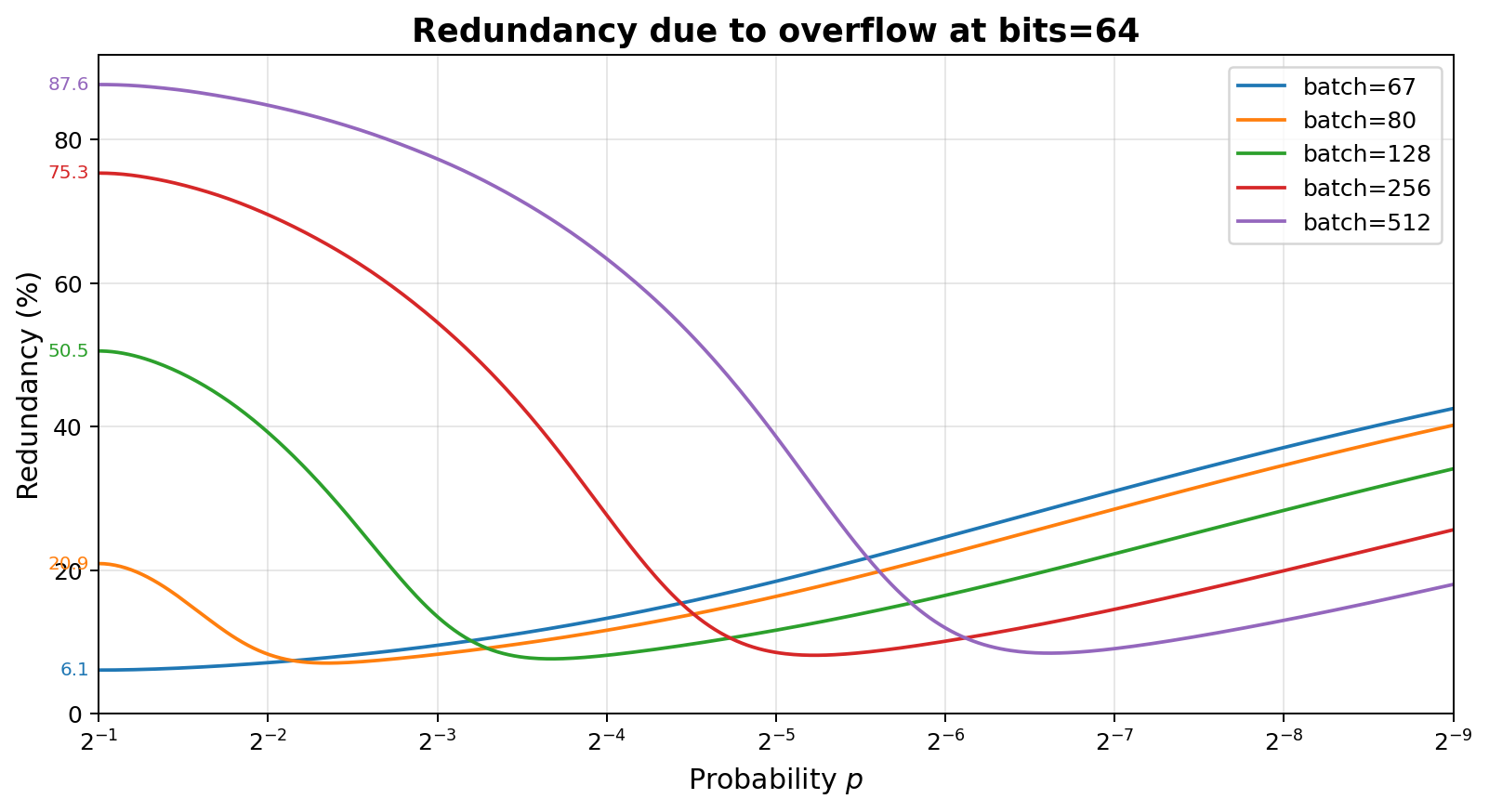
With this change, one can provide arbitrary sized batches to process_batch, even ones that may cause overflow in the final
result, not just in intermediate results. And this may actually be desirable when facing significantly biased inputs,
as shown by this graph. Batch size 67 is the largest which never triggers overflow, and while larger batches show
increasing impact from overflow at low biases, they beat the non-overflowing batch size at high bias.
2.5. Timing side channels
After getting rid of division operations, everything that remains can easily be written in a style that avoids
branches whose runtime may reveal anything about the produced value in uniform spans, or the bits produced
through extract_bit, taking into account that:
-
A constant-time "count trailing zeroes" or "bit scan forward" instruction (or constant-time function) needs to be available in order to implement logic to split integers into an odd + shift form.
-
Bitwise tricks may be needed to avoid branches based on
eventin the batch processing code. extract_bitis not constant time as it has branches that reveal whether overflow triggered, and whether output was produced at all. This is however not secret information; only the produced bit (if any) is secret, and the code path taken reveals no information about that.
The full code implementing all this is provided for C++ as .h and .cpp files.
3. Batch size choice
Everything so far in this document has assumed that event probabilities are unchanging over time, because the alternative violates the i.i.d. assumption of the input, which would result in output bits that are no longer exactly uniformly random.
However, it may be acceptable to use these techniques when the probabilities are known to change very slowly, which may be the case for thermal noise measurements. This is an advantage of Elias and the approach presented here over Peres, as Peres can have a very long memory over which probabilities need to stay fixed. Every batch is processed independently, so there is no requirement that probabilities stay identical across batches in our approach, even when state is carried between batches.
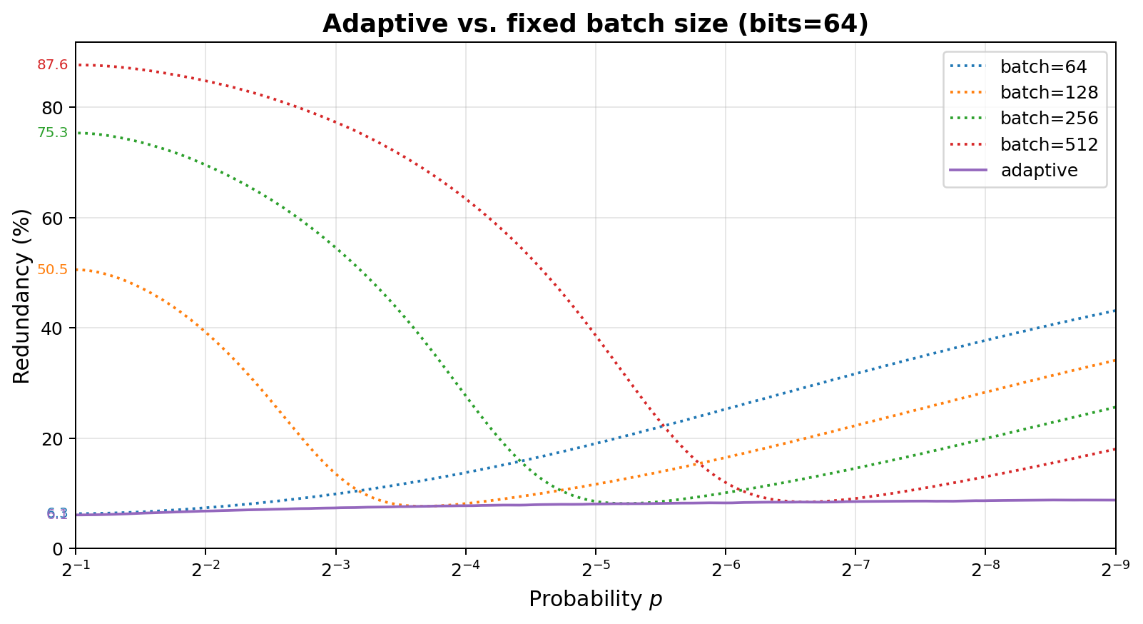
With the overflow protection mechanism introduced above, it also becomes possible to choose batch sizes adaptively as a function of the observed bias of the input, if one takes care to:
-
Decide batch sizes prior to processing a batch, purely based on previous batches. If the batch size is chosen in function of the frequency of events within the batch itself, the resulting spans will no longer be uniform.
-
Make sure the batch size remains negligible compared to the time spans over which probabilities may change.
- Choosing batch sizes based on an inaccurate bias will result in reduced extraction rate (increased redundancy) but will not affect uniformity of the output.
With that, the result is a nearly flat redundancy over a wide spectrum of biases:
When the batches grow large, it may be better to implement the process_batch function(s) incrementally. For the
binary version the only state consists of k, n, value, and span, meaning one does not need to keep all
event values around. The multi-valued version needs event
frequencies instead of k. The C++ code also includes (variable-time) variants that
can be provided just the positions of True events rather than a boolean for every event, which may be desirable
for extremely low $p$.
4. Evaluation
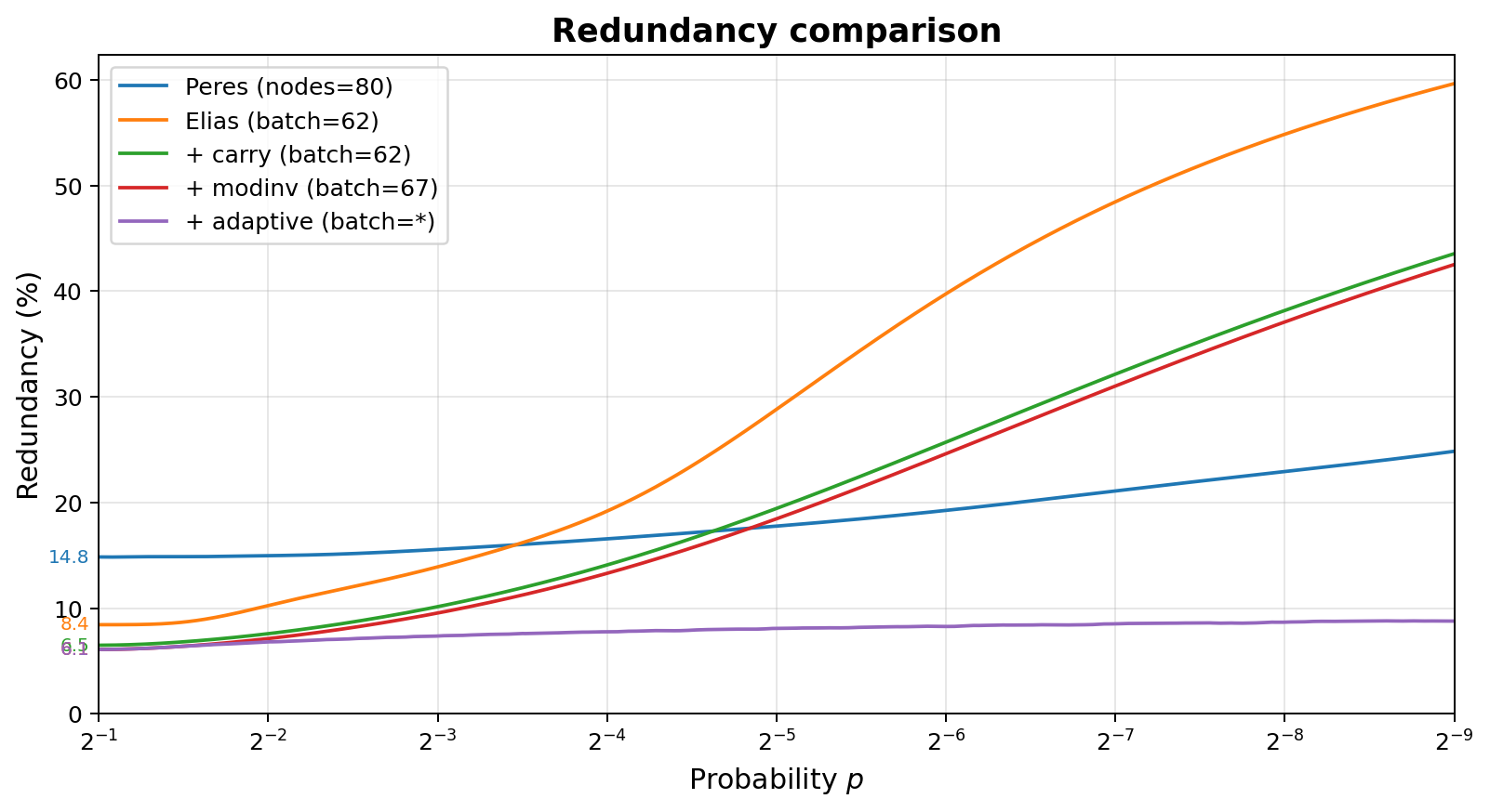
The diagram below shows the redundancy of various techniques, all restricted to 64-bit arithmetic and 160 bits of state (assuming incremental processing of events).
- With Peres (Section 1.2), no arithmetic is needed, but 80 nodes can fit in 160 bits of state.
- With RM based implementation of Elias (Section 1.3, Section 2.1), one is restricted to batches of 62 to avoid overflow.
- Using the modular inverse technique (Section 2.4.1), the limit increases to batches of 67 before overflow causes incorrect results.
- By using overflow protection (Section 2.4.2) and adaptive batch sizes (Section 3), the limit becomes unbounded.
Benchmarks (code) show that modern desktop CPUs can process over 100 million symbols per second, in a single thread, without SIMD, with 64-bit word size and 32-bit carry. For very biased input, with huge batch sizes, it can be a multiple of that.
Acknowledgements
This document and the ideas in it are the result of extensive discussions with Greg Maxwell.
References
- John von Neumann. Various techniques used in connection with random digits. Monte Carlo Method, National Bureau of Standards Applied Mathematics Series, vol. 12, pp. 36–38, 1951.
- Yuval Peres. Iterating Von Neumann's procedure for extracting random bits. The Annals of Statistics, 20(1):590–597, 1992.
- Peter Elias. The efficient construction of an unbiased random sequence. The Annals of Mathematical Statistics, 43(3):865–870, 1972.
- Boris Ya. Ryabko and Elena Matchikina. Fast and efficient construction of an unbiased random sequence. IEEE Transactions on Information Theory, 46(3):1090–1093, 2000.
- Jarosław Duda. Asymmetric numeral systems: entropy coding combining speed of Huffman coding with compression rate of arithmetic coding. arXiv:1311.2540, 2013.
- Henry S. Warren. Hacker's Delight, 2nd edition, page 10-16. Addison-Wesley Professional, 2013.
Changelog
- 2026 Apr 26: converted to a longer explanation post
- 2026 Apr 14: moved here
- 2024 Jun 29: posted as a flat C++ file on GitHub gist (retained as orig_post.cpp here).